Real time ray-tracing was a goal graphics software engineers have sought after ever since the first papers on light simulations were published back in the late 1970s to early 1980s [Whitted 1980][Cook et al. 1984][Veach 1998]. As of now this is no longer a dream, but a reality that is available commercially in modern graphics processing units (GPU) and game consoles such as the PS5 and Xbox Series X.
Real time ray-tracing continues to be a heavily researched topic. From early papers and projects from the demo-scene using shader model 3 to perform simple ray tracing[Quílez 2005], to recent papers running into the issue of branch coherency during acceleration structure traversals [Benthin et al. 2018], attempts to reduce sample counts for rays by means of denoising algorithms. GPU architectural papers such as those released by NVIDIA's Pascal architecture, viewport based quad-tree systems to reduce samples in unimportant areas, BRDF papers for analytically modeling a variety of materials, and so much more, the subject of ray tracing contains a variety of complex sub domains.
While GPUs were originally meant for storing frame buffers, simple rasterization and shading operations, they've since become powerful co-processors that can perform non-specialized calculations, from compute to tensor and ray-tracing routines with varying levels of hardware acceleration. [Arafa 2019]
Thanks to an immense effort on the part of hardware designers, researchers and industry manufacturers, real time hardware accelerated ray tracing is now possible in modern high end graphics cards, with compute based falloffs available on select devices.
Now ray tracing has become an ambiguous term [Shirley 2018] over the years, so let's define terms based on the research papers they were first used:
Ray Casting - a simple collision algorithm, rays can hit a acceleration data structure such as a discrete shape or set of triangles, and that ray returns the data regarding that hit point.
Ray Marching - A method of ray casting that works by "marching" towards a density function's threshold "solid" value [Perlin et al. 1989] by means of a sphere tracing algorithm [Hart et al. 1989]. Similarly, a hierarchical Z Buffer can also be marched, such as in Pixel-projected reflections [Cichocki 2017]. Ray marching has recently been made popular by the DemoScene and ShaderToy.
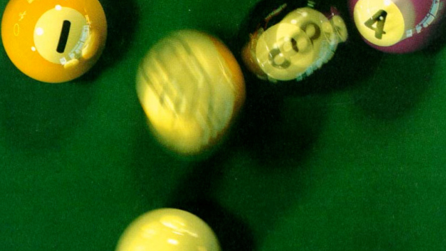
Ray Tracing - otherwise known as Whitted Path Tracing[Whitted 1980] or Recursive Ray Casting, rays can continue past their original collision point, thus allowing for surface behaviors like reflections. Cook Style Ray Tracing (distribution ray tracing) [Cook et al. 1984] involves the use of monte-carlo integration (introducing randomness) on surfaces to introduce soft shadows. The billiard table figure above was rendered with this technique in 1984!
Path Tracing - Kajiya expanded on ray tracing with with the inclusion of diffuse inter-reflection (global illumination) and even further with his light integration formula [Kajiya 1986]. Veach took this even further with his Ph.D dissertation on path tracing which introduced ideas like Multiple Importance Sampling (MIPS), Next Event Estimation (NEE), and Russian Roulette[Veach 1998].
Ray tracing is a subject that can encompass entire books and courses, so it's important to make clear what we won't be discussing in detail:
Acceleration Structures - While KD-Trees and Bounding Volume Hierarchies are important things to know, these are abstracted by real-time Ray Tracing APIs [Stich 2018] (though you could always implement your own, Scratch A Pixel has a brilliant article on the subject, and the subject is detailed in Physically Based Rendering Chapter 4).
Linear Algebra - You should know how to multiply matrices to describe a camera, scene hierarchy, etc. Here's a refresher on the subject.
Overview
The pattern by which any ray based algorithm follows is:
For Each Pixel that you intend to get radiance (light value) information from, cast a ray based on a given camera matrix. This ray can be calculated by getting the NDC coordinate of that pixel, then multiplying that by the inverse view-projection matrix to form a world based vector from the camera to the scene.
Test for Collisions with simple math functions for simple shapes, or more complex methods like a bounding volume hierarchy for traversing the scene, and a low level acceleration structure to test each triangle of the objects in the scene such as a KD-Tree.
Calculate Radiance by testing that surface for its material function (or Bidirectional Reflectance/Transmission Distribution Function, BxDF).
Cast Rays - by bouncing off that surface according to the behavior expected by that material or what you intend to record (Global Illumination, Reflections, etc.).
Stop, Average, and Write at some pre-determined level of quality such as 4096 samples, then average out the radiance values of each of those samples to get a final color. Finally, write that to your output memory, be it a frame buffer attachment in a graphics API or a .png image, etc.
Camera Ray
At the start of every ray tracing routine is the initial camera ray. This can be computed using a View and Projection matrix. If you want to add other effects to your routine such as anti-aliasing or depth of field you can adjust the ray direction with a random offset in its origin and direction.
These matrices can easily be found in linear algebra libraries that include a lookAt and perspective matrix calculation, but the basic idea is to build a basis matrix based on the camera orientation, and a scaling matrix based on its field of view and near/far planes.
Ray Casting is casting a ray from the camera to a collision point and stop the operation there. Early iterations of ray casting were extremely simple, opting to try drawing simple lines or lighting effects.
This is generally a simple operation, and functions as a basic primitive by which all other Ray Tracing methods are built off of.
There's a variety of different operations for triangles and basic primitives, acceleration structures like bounding volume hierarchies, KD-Trees, etc. available here.
Ray Marching
Ray Marching is a form of raycasting that iterates over discrete steps to determine collisions, with Sphere Marching taking that idea a step further, integrating a distance field function to determine collisions (rather than a collision acceleration data structure such as a K-D Tree or Bounding Volume Hierarchy (BVH)). [Hart et al. 1989][Hart 1996][Keinert et al. 2014]
Ray Marching (both terms are used interchangeably) is very useful for rendering real-time volumes, the game Fortnite by Epic Games published a post on FxGuide detailing their technique, and prior to that, Sebastien Hillaire published a paper describing raymarching voxels for volumetric rendering [Hillaire 2015]. Practically every ShaderToy and project in the demoscene uses some form of ray marching.
Note: As ray marching is more of a method of testing collisions, it is possible to use ray marching to drive a ray caster or a complex path tracer.
constint marchSteps = 64;
constfloat epsilon = 1.0e-5;
// ⭕ Sphere Marchingfloat raymarch(vec3 rayOrigin, vec3 rayDirection, float near, float far)
{
// 🏁 Starting integrated distancefloat dist = near + epsilon;
// 📏 Final distance Valuefloat t = 0.0;
// 🥁 Marchfor (int i = 0; i < marchSteps; i++)
{
// 👩🌾 Near/Far Planesif (abs(dist) < near || t > far)
break;
// 🥊 Advance the distance of the last lookup// `dist` approaches values below 0.
t += dist;
vec3 p = rayOrigin + t * rayDirection;
//dist = scenedf(p); // 👈 your scene distance field
}
return t;
}
This can easily be done in a compute or fragment shader with no ray tracing cores necessary.
Ray Tracing is when a ray continues past its original point in a recursive manner. The word tends to be used to describe everything here, recursive ray casts, cook style ray tracing, path tracing, etc.
This is useful to calculate information based on an object's neighbors such as Reflections, Global Illumination or Ambient Occlusion.
Path Tracing
Path Tracing is the process of tracing a ray's path, such as from the camera to a light source. Path tracing is basically ray tracing that uses material functions (BxDFs) to model light interactions and the behavior of rays that interact with those materials.
There are several types of path tracing techniques described in literature, here's a few:
Backwards Path Tracing - Tracing a scene by casting rays from the camera to the scene until they hit light objects. Also called Unidirectional Path Tracing though that title can also apply to only tracing from lights.
Bidirectional Path Tracing - Traditional path tracing, Bidirectional Path Tracing (BPT) where sub paths are started at the camera and the lights (in our case the environment map), and vertices from the sub paths are connected to form a full path.
Importance Sampling
When sampling an environment map, Light, or BxDF, there are regions which are more likely to hit highlights or bright concentrated spots than others, and if you focus your rays to target these regions, you'll see far less variance when sampling these regions.
By varying the local sample density according to the importance function, the error of the approximation can be significantly reduced. The decision whether to place an ink dot is the result of a threshold comparison of each image pixel with the corresponding dither matrix element. [Cornel 2014]
How this is implemented can vary, taking into account Next Event Estimation (NEE), Russian Roulette, and more:
Multiple Importance Sampling (MIPS) - When estimating an integral, we should draw samples from multiple distributions, hoping one matches reasonably well, and weigh the samples from each technique to reduce variance spikes.
Probability Density Function (PDF) - denotes the probability area of a given interaction, which for most of path tracing, is the outgoing direction of a ray according to a BxDF.
Cumulative Distribution Function (CDF) - Usually denoted as ( P(x) ), it's the probability that a uniformly distributed sample ( u < x \int_-\inf^x p(y)dy ). It basically defines the integral of all possible points of a given random variable, and should tend to be 1.0.
Russian Roulette - A random chance that if the luminance of a ray is less than a given ( \epsilon ) the path will be discarded. Reduces variance by accepting stronger rays more often.
Next Event Estimation (NEE) - Tracing shadow rays to the light source on each bounce to see if you can terminate the current path. This involves shooting a shadow ray towards light sources, if it's occluded, terminate the ray.
Conclusion
The differences between ray casting, ray marching, ray tracing, and path tracing are somewhat subtle, it can be useful to imagine each in that order of complexity, with ray casting serving as an operation, ray marching as a method of managing collisions of density functions, and ray tracing serving as an overall description of all techniques.
Professor Morgan McGuire (@CasualEffects) released The Graphics Codex, a massive repository of articles, equations, diagrams, and programming projects.
Compressed-Leaf Bounding Volume Hierarchies Carsten Benthin, Ingo Wald (@IngoWald), Sven Woop and Attila T. Afra High Performance Graphics 2018 ingowald.blog
Hypertexture Ken Perlin and Eric M. Hoffert ACM, SIGGRAPH Computer Graphics 1989 doi.acm.org
[Hart et al. 1989]
Ray Tracing Deterministic 3-D Fractals John Hart, Daniel Sandin and Louis Koffman Siggraph 1989 dl.acm.org
[Cichocki 2017]
Optimized pixel-projected reflections for planar reflectors Adam Cichocki Siggraph, SIGGRAPH Computer Graphics 2017 advances.realtimerendering.com
[Kajiya 1986]
The Rendering Equation James Kajiya ACM, SIGGRAPH Computer Graphics 1986 doi.acm.org
[Stich 2018]
Introduction to NVIDIA RTX and DirectX Ray Tracing Martin Stich NVIDIA Developer Blog 2018 devblogs.nvidia.com
[Hart 1996]
Sphere Tracing: A Geometric Method for the Antialiased Ray Tracing of Implicit Surfaces John Hart The Visual Computer 1996
[Keinert et al. 2014]
Enhanced Sphere Rendering Benjamin Keinert, Henry Schäfer, Johann Korndörfer, Urs Ganse and Marc Stamminger Smart Tools and Apps for Graphics (STAG) 2014 erleuchtet.org
 Alain Galvan ·6/20/2019 8:30 AM · Updated 2 years ago