Alain Galvan ·9/10/2019 8:36 PM · Updated 2 years ago
A review of different techniques for denoising monte-carlo images with machine learning. Learn about autoencoders and currently available implementations such as OIDN and the Optix Autoencoder.
Industry leaders such as Intel and NVIDIA have sponsored research in machine learning based denoisers, Intel Open Image Denoise and the NVIDIA Optix Autoencoder both use a denoising autoencoder to denoise images to great success.
The difficulty in using these lies in their computational cost. Without dedicated hardware or trade offs in quality and performance, it's is difficult to achieve real time high quality denoising using autoencoders.
Thus there's been research in the area of algorithmic techniques to denoise images in real time using spherical harmonics to encode low frequency data, guided filters to blur while avoiding sharp changes in normals or albedo information, and spatio-temporal reprojection to reuse data that isn't view dependent such as global illumination or shadows. [Schied et al. 2019]
There's even ways of combining these two methods, with [Hasselgren et al. 2020] using spatio-temporal methods to feed a sample map estimator network to help dictate how many rays a renderer should dispatch. This helps solve the issue of denoising salt/peppering highlights/shadows in real time. It's also possible to use a different denoising scheme depending on the number of samples in your input such as in [Meng et al. 2020] where 64 spp images were used as input for one of their networks.
Nevertheless It's clear that with images with little history information or with sparse low frequency information, using machine learning results in significantly better quality outputs than algorithmic alternatives such as A-SVGF or custom implementations such as Quake 2/Minecraft RTX's use of split output buffers, upscaling, and spherical harmonics encoding for low frequency data.
It's likely that neural network based denoising solutions will either replace algorithmic techniques or the two will be used in tandem depending on user requirements.
We'll be reviewing machine learning techniques for denoising monte-carlo images, and looking at the state of the art in this area of research.
Autoencoders
An Autoencoder is a neural network that is trained to attempt to imperfectly copy its input to its output. A Denoising Autoencoder take one step further from copying, attempting to learn how to undo the corruption of its input. [Goodfellow et al. 2016]
[R. Alla Chaitanya et al. 2017] makes use of a noisy LDR input, 3 component signed normals,
depth, and roughness to train the autoencoder, with its lack of an albedo channel
most likely the cause of its weakness in estimating the final color of its output.
More recent techniques such as Intel Open Image Denoise and NVIDIA Optix using a
noisy HDR input, 3 component signed normals, and albedo.
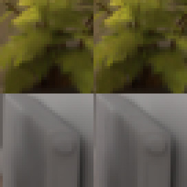
Comparison of an autoencoder trained without and with a GAN by Xu et al. Note sharpness on right.
The most recent state of the art [Li 2020] points to a network being passed the diffuse and specular terms separately like Quake 2 RTX's A-SVGF, and providing auxiliary buffers (Normals, Albedo, Depth) with element wise biasing and scaling of weights. There's a variety of approaches that can be taken to both train and execute the model. Recent literature points to the use of generative adversarial networks (GANs) [Xu et al. 2019] in combination with autonomous reinforcement learning.
Overview
Google TensorFlow, next to Facebook PyTorch, is the most popular neural network framework, so we'll be using TensorFlow to quickly design and train our neural network, then converting our model to DirectML's hardware accelerated machine learning operations, and loading the same weights we calculate with TensorFlow.
We'll be building an autoencoder that takes in the noisy input texture, albedo, view depth, and view normals (with 1st bounce), metalness and gloss (for a total of 12 components), and outputs a single RGBA32 output. This will then be trained using supervised learning on a dataset of monte carlo ray traced images to produce a trained output.
These pixels with 12 components are passed to a series of 2D convolutional neural network layers connected with Leaky Rectifier Linear Activation Units (Leaky RLU) which connect with chunks of the input until it's reduced to a small tensor, then the reverse occurs where convolutions are scaled to a single output.
Perform a initial convolution that reorders inputs
A series of 5 convolutions + max pool operations
5 convolutions + upsample operations
Reordering outputs
This design isn't exclusive to OIDN, NVIDIA's recurrent autoencoder also has 5 downsample convolutions and 5 upsample convolutions, as does Xu et al and Hasselgren et al.
Let's discuss the design of the network, its primitives, and why they're used where they are.
You can find out more about convolutional layers and primitives in Machine Learning in the TensorFlow Guide.
Conv2D
# 🍱🚿 TensorFlowimport tensorflow as tf
from tensorflow.python.keras import layers
layers.Conv2D(filters, kernel_size, ...)
A node that attaches to all subsequent nodes. A Convolution is a function that takes in all the inputs of the previous tensor and connects them with all your specified outputs according to each layer's shape.
This is analogous to a guassian filter in computer graphics. We use this operation to compute weights across a large kernel, similar to how guassian filters compute the average color of a kernel. Operations such as bluring and sharpening an image are convolutions, a matrix operation around a central pixel.
/**
* GLSL Guassian Blur Convolution Example
* By csblo from 🌎 Wikipedia (ShaderToy)
* https://en.wikipedia.org/wiki/Kernel_(image_processing)#Concrete_implementation
* 🎓 Slightly modified for this example:
*/#define gaussian_blur mat3(1, 2, 1, 2, 4, 2, 1, 2, 1) * 0.0625// 🟧 Find coordinate of matrix element from indexvec2 kpos(intindex)
{
returnvec2[9] (
vec2(-1, -1), vec2(0, -1), vec2(1, -1),
vec2(-1, 0), vec2(0, 0), vec2(1, 0),
vec2(-1, 1), vec2(0, 1), vec2(1, 1)
)[index] / iResolution.xy;
}
// 🟥 Extract region of dimension 3x3 from sampler centered in uv// sampler : texture sampler// uv : current coordinates on sampler// return : an array of mat3, each index corresponding with a color channelmat3[3] region3x3(sampler2D sampler, vec2 uv)
{
// ⚪ Create each pixels for regionvec4[9] region;
for (int i = 0; i < 9; i++)
region[i] = texture(sampler, uv + kpos(i));
// 💠 Create 3x3 region with 3 color channels (red, green, blue)mat3[3] mRegion;
for (int i = 0; i < 3; i++)
mRegion[i] = mat3(
region[0][i], region[1][i], region[2][i],
region[3][i], region[4][i], region[5][i],
region[6][i], region[7][i], region[8][i]
);
return mRegion;
}
// 🕸️ Convolve a texture with kernel// kernel : kernel used for convolution// sampler : texture sampler// uv : current coordinates on samplervec3 convolution(mat3 kernel, sampler2D sampler, vec2 uv)
{
vec3 fragment;
// 💉 Extract a 3x3 region centered in uvmat3[3] region = region3x3(sampler, uv);
// 🔴🟢🔵 for each color channel of regionfor (int i = 0; i < 3; i++)
{
// 🔴 get region channelmat3 rc = region[i];
// ∏ component wise multiplication of kernel by region channelmat3 c = matrixCompMult(kernel, rc);
// Σ add each component of matrixfloat r = c[0][0] + c[1][0] + c[2][0]
+ c[0][1] + c[1][1] + c[2][1]
+ c[0][2] + c[1][2] + c[2][2];
// 🔴 for fragment at channel i, set result
fragment[i] = r;
}
return fragment;
}
void mainImage( outvec4 fragColor, invec2 fragCoord )
{
// 📈 Normalized pixel coordinates (from 0 to 1)vec2 uv = fragCoord/iResolution.xy;
// 🕸️ Convolve kernel with texturevec3 col = convolution(gaussian_blur, iChannel0, uv);
// ✍️ Output to screen
fragColor = vec4(col, 1.0);
}
Leaky ReLU
# 🍱🚿 TensorFlowimport tensorflow as tf
from tensorflow.python.keras import layers
layers.LeakyReLU(filters, alpha=.3, ...)
A Leaky Rectifier Linear Unit is an activation function that reduces the magnitude of its input below a threshold value, but otherwise returns a scaled value if it's above the threshold.
This is analogous to:
float x = x < threshold ? x * alpha : x;
We use this to help the neural network find what features it needs to filter, that being areas of high variance in monte carlo images. ReLUs are very good at finding features in stochastic data, but can result in dead neurons in your network, that being, neurons that do not activate.
Max Pool
# 🍱🚿 TensorFlowimport tensorflow as tf
from tensorflow.python.keras import layers
layers.MaxPooling2D(pool_size=(2, 2), ...)
The size of the pooling operation or filter is smaller than the size of the feature map; specifically, it is almost always 2×2 pixels applied with a stride of 2 pixels.
A Max Pooling is a tensor operation that checks neighboring features and outputs the maximum of that area.
This is analogous to downsampling in graphics, where neighboring pixels are often averaged then written to an output smaller than the original as in super-sampled anti-aliasing.
The pattern of convolutions followed by a nonlinear function, followed by pooling is quite common to neural networks. [Brownlee 2019]
Training
Ground Truth
1spp
Direct Normal
Indirect Normal
Indirect Albedo
It's worth noting what data the autoencoder should expect and in what format so it's better tuned for denoising.
Should the autoencoder be able to denoise direct ray data (so direct normals), or direct and indirect (such as reflected normals, reflected albedo, etc.). Intel Open Image Denoise opts for training for both cases, but prefers indirect data as it results in more information for the network to make better decisions with. The decision of which to use can also be ambiguous, as the visibility of indirect rays can depend on the incidence of the first bounce along with their BRDF behavior (imagine capturing normals under a 🚗 car windshield for instance.)
How should you make sure your denoised output is temporally coherent? It's possible to feed motion vectors as an additional feature buffer to help with this.
Is Monte-Carlo biased noise (sobol noise, importance sampling) a factor when training? What about renderers? (Blender Cycles vs. Mitsuba vs. PBRT, etc.)
Should all inputs be anti-aliased or not? Most commercial autoencoders suggest all inputs be anti-aliased, and it is easy to anti-alias ray traced images anyways though offseting samples so this is understandable.
When measuring error, should the variance of the output vs ground truth be used as a metric as error loss, or should the color cosine difference of the output and ground truth be used? It's possible to compare both and determine the best choice by visually comparing models. Xu et al recommends using Wasserstein distance, a probability based distance common to recent GANs.
//https://gist.github.com/mjdietzx/a8121604385ce6da251d20d018f9a6d6
import tensorflow as tf
defem_loss(y_coefficients, y_pred):
return tf.reduce_mean(tf.multiply(y_coefficients, y_pred))
Conclusion
Autoencoders have had great success in denoising images, filling in missing details, and in general getting an image closer to its ground truth.
Here's a few additional resources when developing your own machine learning denoisers:
Xiaoxu Meng released the source
of their Neural Bilateral Grid paper here.
Ingo Wald (@IngoWald) released a Optix course
providing examples for using the Optix denoiser here.
Martin-Karl Lefrançois (@doragonhanta) and
Christoph Kubisch (@pixeljetstream) of NVIDIA
released VKDenoise, an example showcasing
how to denoise a Vulkan scene with the Optix Denoiser.
NVIDIA has released an SDK to itegrate Deep Learning Super Sampling here. AMD's Fidelity FX Super resolution is also available for developers to integrate into their applications.
Memoires associatives distribuees: Une comparaison P. Gallinari, Yann Lecun, S. Thiria and Fogelman F. Soulie Cesta-Afcet 1987 nyuscholars.nyu.edu
[G. Mixon et al. 2018]
SUNLayer: Stable denoising with generative networks Dustin G. Mixon and Soledad Villar ArXiv 2018 deeplearningbook.org
[Khademi Kalantari et al. 2013]
Removing the Noise in Monte Carlo Rendering with General Image Denoising Algorithms Nima Khademi Kalantari and Pradeep Sen Eurographics 2013 research.nvidia.com
[Bako et al. 2017]
Kernel-predicting convolutional networks for denoising Monte Carlo renderings Steve Bako, Thijs Vogels, Brian Mcwilliams, Mark Meyer, Jan Novak, Alex Harvill, Pradeep Sen, T. Derose and Fabrice Rousselle ACM Transactions on Graphics 2017 cvc.ucsb.edu
[Vogels et al. 2018]
Denoising with Kernel Prediction and Asymmetric Loss Functions Thijs Vogels, Fabrice Rousselle, Brian Mcwilliams, Gerhard Rothlin, Alex Harvill, David Adler, Mark Meyer and Jan Novak ACM, ACM Transactions on Graphics 2018 doi.acm.org
[Laine et al. 2019]
Self-Supervised Deep Image Denoising Samuli Laine, Jaakko Lehtinen and Timo Aila CoRR 2019 arxiv.org
[Khademi Kalantari et al. 2015]
A Machine Learning Approach for Filtering Monte Carlo Noise Nima Khademi Kalantari, Steve Bako and Pradeep Sen ACM Transactions on Graphics (TOG) 2015 cvc.ucsb.edu
[R. Alla Chaitanya et al. 2017]
Interactive Reconstruction of Monte Carlo Image Sequences Using a Recurrent Denoising Autoencoder Chakravarty R. Alla Chaitanya, Anton S. Kaplanyan, Christoph Schied (@c_schied), Marco Salvi (@marcosalvi), Aaron Lefohn, Derek Nowrouzezahrai and Timo Aila ACM, ACM Transactions on Graphics 2017 doi.acm.org
[Hasselgren et al. 2020]
Neural Temporal Adaptive Sampling and Denoising Jon Hasselgren, Jacob Munkberg, Marco Salvi (@marcosalvi), Anjul Patney and Aaron Lefohn Eurographics 2020 research.nvidia.com
[Muller et al. 2021]
Real-time neural radiance caching for path tracing Thomas Muller, Fabrice Rousselle, Jan Novak and Alexander Keller Association for Computing Machinery (ACM), ACM Transactions on Graphics 2021 dx.doi.org
[Mildenhall et al. 2017]
Burst Denoising with Kernel Prediction Networks Ben Mildenhall , Jonathan T. Barron, Jiawen Chen, Dillon Sharlet, Ren Ng and Robert Carroll CoRR 2017 arxiv.org
[Lehtinen et al. 2018]
Noise2Noise: Learning Image Restoration without Clean Data Jaakko Lehtinen , Jacob Munkberg , Jon Hasselgren , Samuli Laine , Tero Karras , Miika Aittala and Timo Aila CoRR 2018 arxiv.org
[Dong et al. 2015]
Image Super-Resolution Using Deep Convolutional Networks Chao Dong, Chen Change Loy, Kaiming He and Xiaoou Tang CoRR 2015 arxiv.org
[Ledig et al. 2016]
Photo-Realistic Single Image Super-Resolution Using a Generative Adversarial Network Christian Ledig, Lucas Theis, Ferenc Huszar, Jose Caballero, Andrew P. Aitken, Alykhan Tejani, Johannes Totz, Zehan Wang and Wenzhe Shi CoRR 2016 arxiv.org
[Wang et al. 2018]
A Fully Progressive Approach to Single-Image Super-Resolution Yifan Wang, Federico Perazzi, Brian McWilliams, Alexander Sorkine-Hornung, Olga Sorkine-Hornung and Christopher Schroers CoRR 2018 arxiv.org
[Xiao et al. 2020]
Neural Supersampling for Real-time Rendering Lei Xiao, Salah Nouri, Matt Chapman, Alexander Fix, Douglas Lanman and Anton Kaplanyan Facebook Research 2020 research.fb.com
Real-time Monte Carlo Denoising with the Neural Bilateral Grid Xiaoxu Meng, Quan Zheng, Amitabh Varshney, Gurprit Singh and Matthias Zwicker Eurographics 2020 diglib.eg.org
[Goodfellow et al. 2016]
Deep Learning Ian Goodfellow, Yoshua Bengio and Aaron Courville MIT Press 2016 deeplearningbook.org
Adversarial Monte Carlo Denoising with Conditioned Auxiliary Feature Modulation Bing Xu, Junfei Zhang, Rui Wang, Kun Xu, Yong-Liang Yang, Chuan Li and Rui Tang ACM, ACM Transactions on Graphics 2019 adversarial.mcdenoising.org
[Brownlee 2019]
A Gentle Introduction to Pooling Layers for Convolutional Neural Networks Jason Brownlee 2019 machinelearningmastery.com
 Alain Galvan ·9/10/2019 8:36 PM · Updated 2 years ago
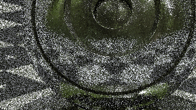 1spp Input
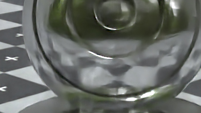 Optix
Optix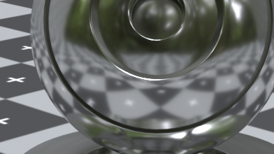 Ground Truth (10K spp)
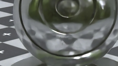 OIDN
OIDN


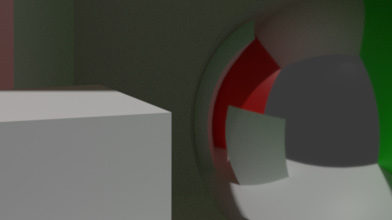 Ground Truth
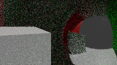 1spp
1spp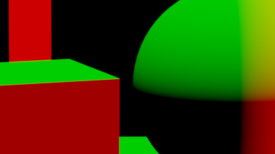 Direct Normal
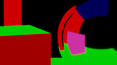 Indirect Normal
 Indirect Albedo
 Riko Ophorst (
 Ingo Wald (
 Martin-Karl Lefrançois (