Alain Galvan ·6/27/2019 9:54 PM · Updated 2 years ago
An overview of image based ray tracing denoising, discussing blurring kernels and spatio-temporal reprojection techniques described in research papers and real time rendering engines.
There's an academic arms race to produce the best real-time denoised image from 1 sample per pixel (spp) path traced images. Every new paper like this brings us closer to an ideal solution that can be baked into silicon (mobile raytacing for the masses!) ~ Dimitri Diakopoulos (@ddiakopoulos)
Since the advent of monte-carlo ray tracing, there have been attempts to reduce the time it takes to converge rays.
This began with algorithms that focused on sampling techniques, using stochastic sampling with biased noise generated by quasi-random sequences, weighing different rays to approximate the best distribution of samples with multiple importance sampling (MIS), Next Event Estimation (NEE), Russian Roulette (RR) [Veach 1998]. Though not necessarily new, recently the use of low discrepancy sampling [Jarosz et al. 2019] and tillable blue noise [Benyoub 2019] has been used by Unity Technologies, and NVIDIA in real time ray tracers to great success.
While this post reviews techniques on improving sampling via filters and noise algorithms, it does not touch improving sampling via modifications to your ray tracing routine with Environment MIS, Ray Sorting, etc. For more details on that visit my other post on Real Time Ray Tracing.
Encoding techniques have been used by recent literature as a means of improving the performance of ray tracing applications by attempting to encode sparsely sampled outputs such as indirect global illumination as 2 levels of spherical harmonics to help avoid salt/peppering, upscaling and finding the best candidate for a ray sample thanks to jittering the frame buffer to better match a given sample to it's closest hit point based on using feature buffers such as normals, depth [Abdollah-shamshir-saz 2018].
Visit my other post on Machine Learning Denoising for more details on implementing an AI denoiser, though these filtering techniques could be used in conjunction with a neural network denoising pass.
Accumulation techniques have seen a resurgence in new literature. While a naive implementation would be to simply accumulate samples on an unchanging scene, it's possible to reuse samples in a moving scene. Examples include [Mara et al. 2017] Spatio-Temporal Filter, the Spatio-Temporal Variance Guided Filter (SVGF) [Schied 2017], Spatial Denoising employed by [Abdollah-shamshir-saz 2018], Adaptive SVGF (A-SVGF) [Schied 2018], Blockwise Multi-Order Feature Regression (BMFR) [Koskela et al. 2019]), and Temporally Dense Ray Tracing [Andersson et al. 2019].
In addition, there's separation techniques that attempt to fine tune behavior for different aspects of a path tracer. The RXGI paper [Majercik et al. 2019] made famous by Morgan McGuire (@CasualEffects) approximated ray traced global illumination (GI) with light probes which used ray tracing to better determine the proper radiance of each probe and to position probes in the scene to avoid bleeding or inaccurate interiors. Specific techniques that can avoid monte carlo integration entirely also avoid the need for real time denoising routines. In addition there have been attempts to move denoising to earlier in rendering by making sampling less biased through ray hashing [Pantaleoni 2020] or using information from spatially and temporally adjacent pixels [Bitterli et al. 2020].
We'll be reviewing techniques that can be used to converge to an image close to ground truth as quickly as possible with real-time ray-tracing renderers. Such denoising techniques can then be applied when rendering shadows, ambient occlusion, global illumination, reflections, refractions, volumetric lighting, and more in your applications.
Execution Order
While there's a variety of ways one could write a ray tracing application and denoiser, the following execution order tends to be the case for the state of the art in real time ray tracing hybrid renderer applications in industry and research:
G-Buffer Pass - Write to feature buffers used commonly for deferred rendering such as view space depth, normals, velocity, or any other feature sets you intend on using when denoising.
Ray Trace - Either with a unified path tracer or using dedicated passes for shadows/reflection/global illumination/ambient occlusion/subsurface scattering/refraction/translucency. Having each aspect of your ray tracer split however can allow for separate denoising schemes that work best for each type of output, though it could be slower.
Accumulation - by interpolating between previous and current color data. Normally this involves reprojecting previous samples, though [Kristof 2019] attempts to reproject previous samples first for reflections (so switching steps 2 and 3), then use that data to guide accumulation.
Blit Accumulation History - write your accumulated buffers to be used by the next frame when spatially reprojecting samples. It's important to do this before any filtering to prevent a growing blur effect as every frame blurs the previous.
Adaptive Heuristics - A-SVGF introduces the Moment Buffer that encodes change in color variance/velocity to better avoid using old history on areas that have a lot of changes such as moving lights, mirrors, etc. By estimating the current radiance of your path traced image, you can also take advantage of that data to perform firefly rejection.
Guided Filtering - Blur the weighting buffers using a guided filter such as À-Trous, or an edge stopping Gaussian filter. Most denoisers do this 5 times with a 3x3 filter. This can also be guided by the change in velocity/luminance, history length, roughness, shadow penumbra distance, etc.
Blit Prepass History - Write any important previous data sets (linear depth, normals, velocity), preferably by ping-ponging between two output frame buffers to save a copy operation. These will be used for accumulation and reprojection on the next frame.
Sampling Techniques
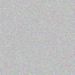
One of the easiest and fastest ways to get an image to converge faster is to use low discrepancy noise when performing monte-carlo integration. This is better than using purely random noise due to it having a more uniform distribution. This means that the random samples cover the sample domain evenly, rather than cluster and form holes. [Cornel 2014]
The faster an image converges, the less variance your data will have when feeding it to a denoiser. However, it's important to bare in mind the Curse of Dimensionality:
Once the integral is high dimensional, if the integrand is complex, Stratified Sampling doesn't help. ~ Peter Shirley (@peter_shirley)
Thus, try to keep the integrand of your ray trace as minimal or as full of constants as possible. [Shirley 2018]
Blue Noise
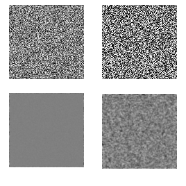
Blue noise is uniformly distributed noise, that is noise with similar samples spread out as far away as possible over a given domain. This lends itself very well to denoising, as there are far less instances of high frequency error in blue noise, making it easier to blur and accumulate [Schied et al. 2019].
Once you have a uniform Blue Noise Look Up Texture (LUT) (sometimes called a precomputed dither matrix in literature) to work with, it's possible to map that texture to important regions to sample during ray tracing, such as the BRDF behavior of a given surface and/or the bright regions of an environment texture in the case of image based lighting.
Blurring blue noise even a little (in this case a 2x gaussian blur) results in a much more uniform result in comparison with white noise where high frequency noise present in monte-carlo rendering would be much more obvious.
Though it should be noted that it can be difficult to blur across edges, especially with temporal anti-aliasing with the previous history buffer may not be accurate to your current viewport to to the perspective pixel shift involved.
Sobol Sequences
Computing blue noise is a somewhat expensive and thus, is only suitable to compute in a preprocessing step. There do however exist functions that behave similarly to blue noise, known as quasi-random number sequence algorithms. Examples include the Worley, Sobol, or Halton Sequences, each of which have benefits and tradeoffs [Wolfe 2017].
Sobol is more computationally expensive but leads to far less discrepancy [Roberts 2018], while Halton is cheaper but has slightly more discrepancy [Wong et al. 1997].
Anis Benyoub (Unity Technologies) for instance has chosen to use a 256x1 Sobol texture and a 256x256 RG Blue Noise texture as a means of generating quasi-random monte-carlo (QMC) samples. [Benyoub 2019]Eric Heitz (@eric_heitz) et al. took this even further with his paper on distributing monte carlo errors over different frames by using a uint sobolSequence[256*256] to scramble blue noise tiles. [Heitz et al. 2019]
A C++ implementation of Sobol can be found here, courtesy of Professor John Burkardt of Virginia Tech.
Having a low discrepancy domain from which to sample your scene can then be used in combination with other techniques such as Multiple Importance Sampling (MIS) of the BRDF (material) behavior and light source behavior (with environment maps and participating media being different cases to consider), Next Event Estimation, Russian Roulette, all with the goal of reducing the variance of a monte-carlo raytraced image.
For more details regarding these techniques, visit my post on Real Time Raytracing.
Encoding Techniques
Formats
When managing a real time ray tracing application, the question of what formats to use with your trace output buffers will ultimately come into play. The answer to such a question ultimately boils down to:
Are you targeting an HDR output such as with ACES linearization or an HDR 10 bit display, or a 16 bit or 32 bit output image.
How many samples you wish to accumulate, as there's a limit to where averaging out samples over time no longer contribute to the output image, and a small enough limit where they introduce bias to your image that can lead to color banding.
This sample count limit can be defined as:
Samples1≥ϵbitrate
The limit where the number of samples you've accumulated is less than the minimum ( \epsilon ) of your floating point bit rate. For RGBA16F that number is about 2048 samples. [Wolfe 2017]
On a side note, formats such as R11G11B10 are not recommended due to any accumulation of samples ultimately having a bias towards turning yellow due to the extra precision on the R and G channels.
Spherical Harmonics
Rather than writing sparse samples as radiance in a 1 pixel location, it's possible to write such samples as spherical harmonics encodings across a larger radius that does not intersect with other samples, and use filtering to fill in the gaps.
Upscaling
Raytracing is an expensive operation to be done at high resolutions such as Ultra HD 4K, so upscaling from a lower resolution can be employed to take advantage of raytracing at interactive frame rates.
Spatio-Temporal Techniques
Spatiotemporal reprojection is simply reusing the data from previous frames, spatially reprojecting them to the current frame. Encoding radiance with spatial information has had its earliest literature in Irradiance Caching[Ward et al. 1988], however real time raytracing takes this idea a step further by keeping data in view space, but attempting to reuse that data by translating it from one frame to the other by means of a motion buffer which calculates the change in a vertex's position between the current and previous frame.
This is extremely effective at reducing noise, but relying on temporal data inevitably introduces a slight lag with changes in a scene such as moving lights, objects, as new data needs to be accumulated over time to reflect those changes.
Motion Buffer
A Motion Buffer (otherwise known as a Velocity Buffer) encodes the change in position of each vertex. This is at the core of spatio-temporal reprojection. This buffer can be calculated by determining the previous and current NDC space coordinate positions of each vertex being rendered, and taking the difference of the two. This can be encoded in a RG16F render target.
V=NDCcur−NDCprev
Therefore, one would need the previous modelViewProjection matrix of an object, as well as that object's animation vertex velocity, the difference between the position between the current and previous animation sample.
When performing spatio-temporal reprojection, having a buffer describing the time for which a given sample had to accumulate is very valuable, a History Buffer. It can be used to drive a filter to blur stronger in regions with few accumulated samples or be used to estimate the variance of the current image (higher history would mean less variance).
This buffer would be read when accepting reprojected samples to determine the accumulation factor of a given sample with an exponentially moving average.
Having a history buffer available to you gives your algorithm a perspective of how many samples a given region of the screen have been accumulated, which you can feed to a shader to determine an accumulation factor ( \alpha ).
While this can encode spatial information thanks to the motion buffer allowing for the translation of previous samples, A-SVGF takes this a step further.
Moment Buffer
By using the change in luminosity and velocity over correlated samples to help drive the accumulation factor of a spatio-temporal filter, it's possible to reduce ghosting significantly.
This difference in temporal variance and velocity is then used to determine the rate of change on a sample of the screen, encoding that information in what it calls a Moment Buffer. [Schied et al. 2019]
We'll discuss an implementation of a moment buffer while discussing variance estimation later in the post.
Caveats
Temporal lag is a problem with this technique. There can be differences in brightness between regions with a high number of accumulated samples and new regions. This is especially evident in darker regions of a raytraced scene such as interiors. To mitigate this, rather than using 1 sample per pixel, it's best to use 2 or more samples per pixel in dark areas of a scene.
In addition, there can be significant differences between view positions and their ray traced outputs. While shadows, global illumination, ambient occlusion, subsurface scattering, and translucency can be reprojected spatially without much issue, ray traced outputs that are not lambertian in nature such as reflections and refraction cannot be reprojected (at least, without taking into account bounce velocity, which may be more computational trouble than its worth and not yield many reprojected samples). Thus, these buffers would rely much more on filtering techniques.
Signal Processing Techniques
Monte-carlo integration starts with a noisy image which gradually becomes clearer as time goes on. In an attempt to reduce the amount of time it takes to compute a clear final image, attempts have been made to use a variety of filtering techniques when rendering such as Gaussian, Median, Bilateral, and À-Trous filters. These have been used in combination with variance estimation across neighboring samples to better reject fireflies and drive the accumulation of samples in regions that change in variance/velocity.
Bluring Kernels
Filtering is an expensive operation to do in a real-time renderer, as texture lookup operations introduces latency when executing a shader. À-Trous (With holes) is a fast approximation of a bilateral filter currently used by Spatio-temporal Variance Guided Filtering (SVGF) and it's Adaptive (A-SVGF) counterpart [Schied 2017][Schied 2018], first introduced in [Dammertz et al. 2010], in combination with spatio-temporal reprojection and variance estimation to perform a cheap, fast, and high quality edge avoiding blur.
Normals (RG16F)
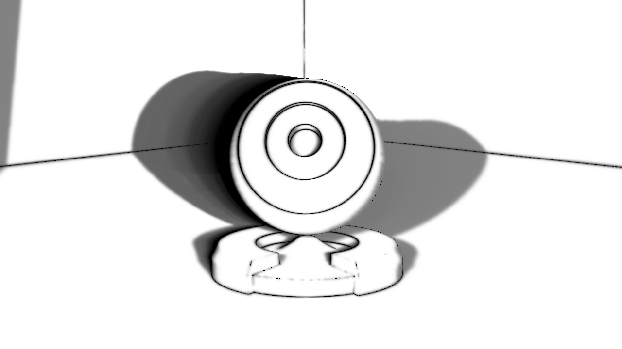
View Space Depth (R32F)
A-Trous avoids sampling in a slightly dithered pattern to cover a wider radius than would normally be possible in a 3x3 or 5x5 guassian kernel while at the same time having the ability to be repeated multiple times, and avoid bluring across edges thanks number of different inputs [He et al. 2012][Li et al. 2012][Dammertz et al. 2010], such as a Normals, Depth, Squared World Space Positions, derivatives of said attachments [Koskela et al. 2019], the change in variance of luminosity, and change in velocity of those buffers [Schied 2018].
This can be done in combination with:
Subsampling according to a dithering pattern, thus reducing the number of samples in your bluring kernel even more.
Noise Dancing is more prominant and visible when it's blured, especially if your integrand is complex enough.
Balancing your blurring size with keeping high frequency details is a diffcult problem, with Machine Learning kernels doing better than variance guided filters.
Variance Estimation
σ2=nΣ(x−x^)2
Variance is the squared difference of a signal's average (mean). One can take the average of the current signal and that signal squared with a 3x3 gaussian kernel, then taking the difference of the two.
σ2=nΣx2−x^2
constfloat radius = 2; //5x5 kernelvec2 sigmaVariancePair = vec2(0.0, 0.0);
float sampCount = 0.0;
for (int y = -radius; y <= radius; ++y)
{
for (int x = -radius; x <= radius; ++x)
{
// ☝️ We already have the center dataif (xx != 0 || yy != 0) { continue; }
// ⬇️ Sample current point data with current uvivec2 p = ipos + ivec2(xx, yy);
vec4 curColor = texelFetch(tColor, p, 0);
// 💡 Determine the average brightness of this sample// 🌎 Using International Telecommunications Union's ITU BT.601 encoding paramsfloat samp = luminance(curColor);
float sampSquared = samp * samp;
sigmaVariancePair += vec2(samp, sampSquared);
sampCount += 1.0;
}
}
sigmaVariancePair /= sampCount;
float variance = max(0.0, sigmaVariancePair.y - sigmaVariancePair.x * sigmaVariancePair.x);
Christoph Schied (@c_schied) does this in A-SVGF estimating the spatial variance as a combination of an edge avoiding guassian filter (just like in the a-trous guided filter) and using this in a feedback loop to drive the accumulationFactor during spatio-temporal reprojection:
/**
* Variance Estimation
* Copyright (c) 2018, Christoph Schied
* All rights reserved.
* 🎓 Slightly simplified for this example:
*/// ⛏️ Setupfloat weightSum = 1.0;
int radius = 3; // ⚪ 7x7 Gaussian Kernelvec2 moment = texelFetch(tMomentPrev, ipos, 0).rg;
vec4 c = texelFetch(tColor, ipos, 0);
float histlen = texelFetch(tHistoryLength, ipos, 0).r;
for (int yy = -radius; yy <= radius; ++yy)
{
for (int xx = -radius; xx <= radius; ++xx)
{
// ☝️ We already have the center dataif (xx != 0 || yy != 0) { continue; }
// ⬇️ Sample current point data with current uvivec2 p = ipos + ivec2(xx, yy);
vec4 curColor = texelFetch(tColor, p, 0);
float curDepth = texelFetch(tDepth, p, 0).x;
vec3 curNormal = texelFetch(tNormal, p, 0).xyz;
// 💡 Determine the average brightness of this sample// 🌎 Using International Telecommunications Union's ITU BT.601 encoding paramsfloat l = luminance(curColor.rgb);
float weightDepth = abs(curDepth - depth.x) / (depth.y * length(vec2(xx, yy)) + 1.0e-2);
float weightNormal = pow(max(0, dot(curNormal, normal)), 128.0);
uint curMeshID = floatBitsToUint(texelFetch(tMeshID, p, 0).r);
float w = exp(-weightDepth) * weightNormal * (meshID == curMeshID ? 1.0 : 0.0);
if (isnan(w))
w = 0.0;
weightSum += w;
moment += vec2(l, l * l) * w;
c.rgb += curColor.rgb * w;
}
}
moment /= weightSum;
c.rgb /= weightSum;
varianceSpatial = (1.0 + 2.0 * (1.0 - histlen)) * max(0.0, moment.y - moment.x * moment.x);
outFragColor = vec4(c.rgb, (1.0 + 3.0 * (1.0 - histlen)) * max(0.0, moment.y - moment.x * moment.x));
Firefly Rejection
Firefly rejection can be done in a variety of ways, from adjusting how you're sampling during raytracing, to using filtering techniques or huristics about your output radiance.
Denoising results in a drastic difference in the quality of a given image. By using a combination of advanced sampling, encoding, accumulation, and filtering techniques, it's possible to achieve very high quality images for the small price of a few ms.
Aspects of this can also be driven by machine learning algorithms, which can serve as a smarter bluring tool than a bilateral filter, or trained to temporally accumulate samples faster. There's plenty of room for future work here!
Here's a few additional example implementations of real time ray tracing denoisers worth reviewing in no particular order:
Peter Kristof of Microsoft made a really robust RTX Ambient Occlusion example with a robust implementation of SVGF here.
Christof Shied (@c_schied) and Alexey Panteleev of NVIDIA wrote the denoiser for Quake 2 RTX (which is referenced heavily in this post) which is on Github here.
Ingo Wald (@IngoWald) released a Optix course providing examples for using the Optix denoiser here.
Robust Monte Carlo Methods for Light Transport Simulation Eric Veach Stanford University 1998 graphics.stanford.edu
[Jarosz et al. 2019]
Orthogonal array sampling for Monte Carlo rendering Wojciech Jarosz (@wkjarosz), Afnan Enayet, Andrew Kensler, Charlie Kilpatrick and Per Christensen EGSR 2019 cs.dartmouth.edu
Edge-Avoiding À-Trous Wavelet Transform for fast Global Illumination Filtering Holger Dammertz (@NeoSpark314), Daniel Sewtz, Johannes Hanika and Hendrik P.A. Lensch High Performance Graphics 2010 jo.dreggn.org
[He et al. 2012]
Guided Image Filtering Kaiming He, Jian Sun and Xiaoou Tang 2012 kaiminghe.com
[R. Alla Chaitanya et al. 2017]
Interactive Reconstruction of Monte Carlo Image Sequences using a Recurrent Denoising Autoencoder Chakravarty R. Alla Chaitanya, Anton S. Kaplanyan, Christoph Schied (@c_schied), Marco Salvi (@marcosalvi), Aaron Lefohn, Derek Nowrouzezahrai and Timo Aila ACM 2017 research.nvidia.com
[Khademi Kalantari et al. 2015]
A Machine Learning Approach for Filtering Monte Carlo Noise Nima Khademi Kalantari, Steve Bako and Pradeep Sen ACM Transactions on Graphics (TOG) 2015 cvc.ucsb.edu
Dynamic Diffuse Global Illumination with Ray-Traced Irradiance Fields Zander Majercik, Jean-Philippe Guertin, Derek Nowrouzezahrai and Morgan McGuire (@CasualEffects) 2019 jcgt.org
[Pantaleoni 2020]
Online Path Sampling Control with Progressive Spatio-Temporal Filtering Jacopo Pantaleoni NVIDIA 2020 arxiv.org
 Alain Galvan ·6/27/2019 9:54 PM · Updated 2 years ago


 History (R16 Normalized [0, 212])
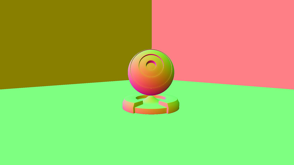 Normals (RG16F)
 View Space Depth (R32F)
 Ingo Wald (