Ray Tracing Denoising

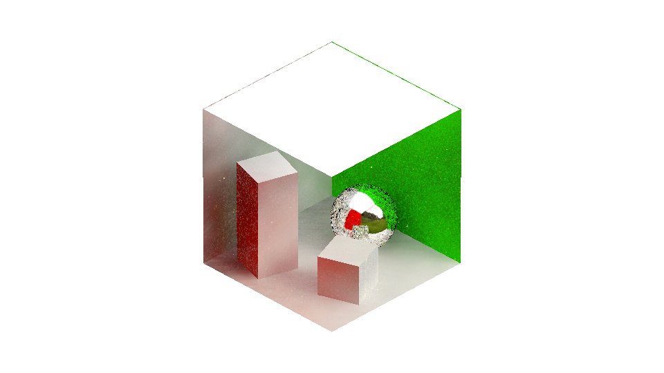
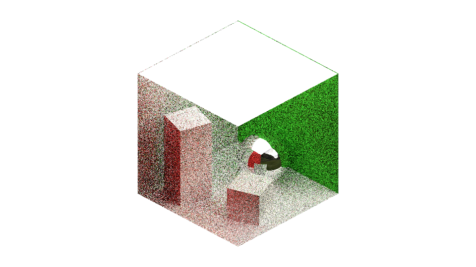
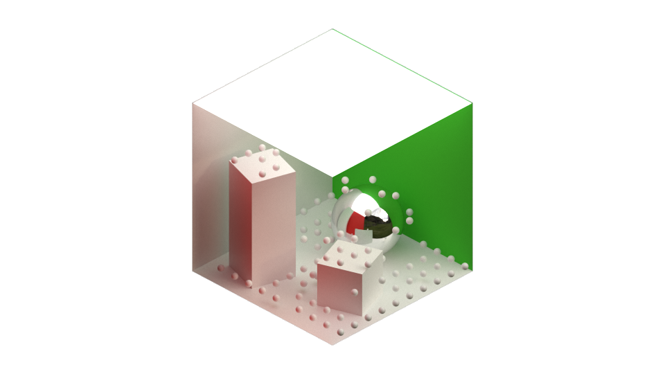
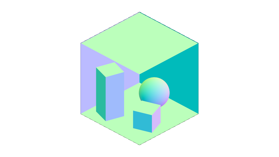
Monte-carlo ray tracing is a technique that relies on accumulating random samples to reach a satisfying approximation of a given scene. This process was traditionally a slow one with plenty of variance, but with the advent of real time ray tracing solutions with recent graphics cards, there's been a resurgence of research in denoising techniques.

These denoising techniques include filtering using guided blurring kernels, machine learning to drive filters or importance sampling, improving sampling schemes through better quasi-random sequences such as blue noise and spatio-temporal reuse of either rays or the final luminance, and approximation techniques that attempt to quantize and cache information with some sort of spatial structure such as probes, irradiance caches, neural radiance fields (NeRFs), etc.

A robust denoiser should consider using all of these techniques depending on the trade-offs and needs of your application.

Recent research has focused on moving denoising to earlier in rendering by improving sampling schemes and re-sampling pixels with cached information, with prior research focused on filtering, autoencoders in machine learning, importance sampling, and real time methods that are currently in production in commercial games and renderers. We'll be discussing key papers on denoising and their implementations, focusing on how to build your own robust real time ray tracing denoiser.

Denoising has seen a significant number of new publications since the release of this article, with techniques such as ReSTIR, NVIDIA's denoising suite, and machine learning techniques improving significantly. This article could use some updates for these recent papers, but the ideas here are still applicable today.

Prior Art

Filtering techniques such as Gaussian, Bilateral, À-Trous [Dammertz et al. 2010], Guided [He et al. 2012], and Median [Mara et al. 2017] filters have been used to blur monte-carlo ray traced images. In particular Guided filters driven by feature buffers such as common G-Buffer attachments in Deferred Rendering like normals, albedo, depth/position, as well as specialized buffers such as first-bounce data, reprojected path length, or view position have been used in recent denoising papers and commercial implementations.

While these filtering techniques are effective and cheap to compute, they come at the cost of a lossy representation of the scene and the reduction of high frequency information like sharp edges. This loss of information can be so drastic that it can even lead to differences in the level of brightness in scenes with salt & peppering occurring in either highlights or shadows.

Machine Learning has been used in a wide range of problem domains related to denoising, from general image reconstruction to real time ray tracing denoising through the use of denoising autoencoders [Khademi Kalantari et al. 2013] [Khademi Kalantari et al. 2015] [R. Alla Chaitanya et al. 2017] [Vogels et al. 2018], driving filtering techniques [Wang et al. 2018] [Xu et al. 2019] [Meng et al. 2020] [Işık et al. 2021], varying convolution sizes to reduce computational costs [Jiang et al. 2022], spatio-temporal techniques [Hasselgren et al. 2020], NeRFs to approximate view dependent effects like reflections [Verbin et al. 2021] or to denoise a scene [Mildenhall et al. 2022], and upscaling images while maintaining detail through super-resolution/super-sampling [Dong et al. 2015] [Ledig et al. 2016] [Xiao et al. 2020]. Denoising and supersampling can even be done together using a neural network [Mathew Thomas et al. 2022], with NVIDIA integrating both in DLSS 3.5.

Industry leaders such as Intel and NVIDIA have sponsored research in machine learning based denoisers, Intel Open Image Denoise and the NVIDIA Optix Autoencoder both use a denoising autoencoder to denoise images to great success. NVIDIA's Deep Learning Super Sampling (DLSS 2.0) has also been used to upscale ray traced applications such as Minecraft RTX, Remedy Entertainment’s Control, and more, with the goal of reducing computational costs by upscaling to native resolutions a fraction of the original image.

Sampling techniques have seen a resurgence in new literature. While a naive monte carlo ray tracer would simply accumulate samples on an unchanging scene, it's possible to reuse samples in a moving scene. Examples include Temporal Anti-Aliasing [Korein et al. 1983] [Yang et al. 2020], the Spatio-Temporal Filter [Mara et al. 2017], the Spatio-Temporal Variance Guided Filter (SVGF) [Schied 2017], Spatial Denoising employed by [Abdollah-shamshir-saz 2018], Adaptive SVGF (A-SVGF) [Schied et al. 2018], Blockwise Multi-Order Feature Regression (BMFR) [Koskela et al. 2019]).

These techniques would rely on using high frequency quasi-random sequences such as blue noise (which would be used in combination with filtering) [Benyoub 2019] , as well as common tools such as firefly rejection [Liu et al. 2019], next event estimation (NEE), and importance sampling [Veach 1998].

There have also been attempts to move denoising to earlier in rendering by making sampling less biased through ray hashing [Pantaleoni 2020] or reusing statistics from neighboring sampling probabilities [Bitterli et al. 2020]. Variations of these techniques have emerged that target a smaller subset of ray tracing such as Global Illumination [Boisse 2021] and motion blur [Oberberger et al. 2022], or using tiles for point lights [Tokuyoshi 2022].

In addition, there's approximation techniques that attempt to fine tune behavior for different aspects of a path tracer. The RTX Global Illumination paper approximated ray traced global illumination (GI) with light probes which used ray tracing to better determine the proper radiance of each probe and to position probes in the scene to avoid bleeding or inaccurate interiors. Techniques that can avoid screen space monte carlo integration entirely such as RTXGI also avoid the need for real time denoising routines but can be used together with screen space techniques. RTXGI have been recently integrated to commercial game engines such as Unreal Engine 4 and Unity [Majercik et al. 2020].

Sampling

SVGF

The Spatio-Temporal Variance Guided Filter (SVGF) [Schied 2017] is a denoiser that uses spatio-temporal reprojection along with feature buffers like normals, depth, and variance calculations to drive a bilateral filter to blur regions of high variance.

Minecraft RTX uses a form of SVGF, with the addition of irradiance caching, the use of ray length for better driving reflections, and splitting rendering for transmissive surfaces such as water. SVGF, while very effective, does introduce temporal lag that is noticable in game.

A-SVGF

Adaptive Spatio-Temporal Variance Guided Filtering (A-SVGF) [Schied et al. 2018] improves on SVGF by adaptively reusing previous samples that have been spatially reprojected according to temporal hueristics such as the change in variance, viewing angle, etc. encoded in a Moment Buffer, and filtering that with a fast bilateral filter. So rather than accumulating samples based on history length, the moment buffer acts as an alternative hueristic that uses the change in variance to drive the proportion of old samples and newer samples, resulting in less ghosting. While SVGF only used the moment buffer to drive blurring, A-SVGF uses it for both the filtering and accumulation steps.

Though the introduction of a moment buffer helps with temporal lag it doesn't completely get rid of it. There can be differences in brightness between regions with a high number of accumulated samples and new regions. This is especially evident in darker regions of a raytraced scene such as interiors. To mitigate this, rather than using 1 sample per pixel (1 spp), it's best to use 2 spp in dark areas of a scene.

Quake 2 RTX uses A-SVGF as its denoising solution.

ReSTIR

Spatiotemporal Importance Resampling for Many-Light Ray Tracing (ReSTIR) [Bitterli et al. 2020] attempts to move the spatio-temporal reprojection step of real time denoisers to earlier in rendering, reusing statistics from neighboring sampling probabilities. This is essentially a combination of an earlier paper by [Talbot et al. 2005] discussing Resampled Importance Sampling, and adding ideas introduced by spatio-temporal denoisers.

ReSTIR will be available for use in NVIDIA's RTXDI SDK.

Machine Learning

These remarkable results show yet another example of how rapidly DNNs are finding their place in and evolving modern renders. ~ Marco Salvi (@marcosalvi)

Machine learning techniques such as denoising autoencoders, sample map estimators driving sample counts or importance sampling, neural bilateral grids driving filtering, and super-sampling result in the most drastic improvements in image quality, though these techniques are slower than other algorithms such as A-SVGF.

Intel OIDN

Intel Open Image Denoise (OIDN) is a machine learning autoencoder that takes in a albedo, first bounce normals, and your input noisy image and output a filtered image.

// 👋 Declare Handles

// Images loaded from stb as 3 components
float* color;
float* normal;
float& output;
unsigned width;
unsigned height;

oidn::DeviceRef device = oidn::newDevice();
device.commit();
oidn::FilterRef filter = device.newFilter("RT");
filter.setImage("color", color, oidn::Format::Float3, width, height);
filter.setImage("normal", normal, oidn::Format::Float3, width, height);
filter.setImage("output", output, oidn::Format::Float3, width, height);
filter.set("hdr", true);
filter.commit();
filter.execute();

NVIDIA Optix

NVIDIA's Optix 7 Denoising Autoencoder [R. Alla Chaitanya et al. 2017] takes in the same inputs as OIDN, an optional albedo, normal, and input noisy image, and outputs a filtered image much faster than Intel's solution at the cost of quality.

// 👋 Declare Handles
OptixContext ctx;
OptixDevice device;
unsigned width;
unsigned height;
CUDABuffer denoiserState;
CUDABuffer denoiserScratch;

// https://github.com/ingowald/optix7course/blob/master/example12_denoiseSeparateChannels/SampleRenderer.cpp#L764
OptixDenoiser denoiser;
OptixDenoiserOptions opt;
opt.inputKind = OPTIX_DENOISER_INPUT_RGB_ALBEDO;
opt.pixelFormat = OPTIX_PIXEL_FORMAT_FLOAT4;
optixDenoiserCreate(ctx, &opt, &denoiser);
optixDenoiserSetModel(denoiser, OPTIX_DENOISER_MODEL_KIND_HDR, nullptr, 0);
OptixDenoiserSizes denoiserReturnSizes;
optixDenoiserComputeMemoryResources(denoiser, width, height, &denoiserReturnSizes);
denoiserState.resize(denoiserReturnSizes.stateSizeInBytes);
optixDenoiserSetup(denoiser,0,
                width, height,
                denoiserState.d_pointer(),
                denoiserState.size(),
                denoiserScratch.d_pointer(),
                denoiserScratch.size());

DLSS

Deep Learning Super Sampling (DLSS) is an upscaling technique that that uses a small color buffer and a direction map to multiply the resolution of the output 2-4 times. This is exclusive to developers pre-approved by NVIDIA, so there's currently no way to use this publicly, that being said there's alternatives such as DirectML's SuperResolution Sample.

Denoiser Design

An ideal denoiser that combines ideas from the latest state of the art papers could look like the following:

1. Prepass - Calculate the NDC space velocity of the scene, write common G-Buffer attachments such as albedo, normals etc. You may also want first bounce versions of those buffers, which would require a ray-trace based prepass rather than a raster based one.

2. Ray Trace - Use AI Adaptive sampling from [Kuznetsov et al. 2018] [Hasselgren et al. 2020] with a sample map to better determine which regions should recieve more samples, generally highlights/shadows to help avoid salt/peppering and maintain luminance over time. A split denoiser with Specular Reflections and Global Illumination written to separate attachments would be ideal as Reflection denoising would do better 1st bounce data, Global Illumination/Ambient Occlusion/Shadows can afford to use simpler spatio-temporal accumulation based off less data.

3. Accumulation - Use Spatio-Temporal Reprojection as often as possible, this is easier to do with lambertian data such as Global Illumination/Ambient Occlusion, and harder with specular data like reflections. For better results, use heuristic data like normals/albedo/object IDs to translate previous samples to the current position, as well as 1st bounce data such as view direction, 1st bounce normals/albedo, etc. Any successful reprojections can then be used to either importance sample [Bitterli et al. 2020] or their radiance encoded to a radiance history buffer [Schied et al. 2018].

4. Statistical Analysis - estimate the variance of the current ray traced image, calculate the change in variance in luminance/velocity and use that to drive spatio-temporal reprojection and filtering. Attempt to reject fireflies with that variance information.

5. Filtering - This can be done quickly with an À-Trous bilateral filter, repeat this step 3-5 times depending on how strong of a blur you want, and decrease the stepWidth by a power of 2 each time (so a sequence of 4, 2, 1 in the case of 3 iterations). Alternatively, you could use a denoising autoencoder which will be slower, but can produce better filtering results. That result could then be fed into a super sampling autoencoder that could upscale your results, similar to NVIDIA's DLSS 2.0.

6. History Blit - Write the current prepass data such as Albedos, Depth, etc. for reprojection next frame.

NVIDIA released an example implementation of a denoiser similar to this that uses ReSTIR [Wyman et al. 2021].

Prepass

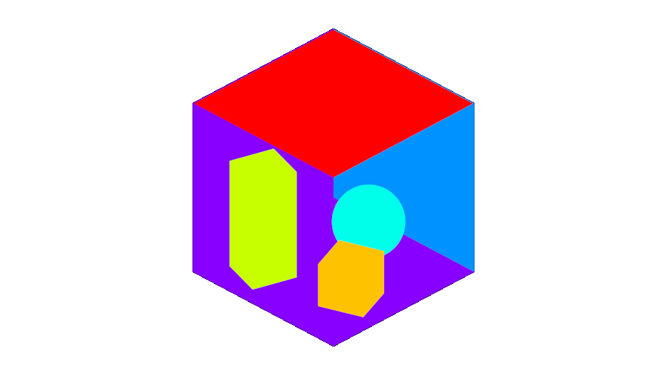
Prior to denoising, it's important to encode material information such as Normals, Albedo, Depth/Position, Object ID, Roughness/Metalness, etc. with some sort of General Pass (G-Pass). In addition, having access to velocity makes it possible to translate previous samples to the current position.

A Velocity Buffer can be calculated by determining the previous and current NDC space coordinate positions of each vertex being rendered, and taking the difference of the two.

Therefore, one would need the previous modelViewProjection matrix of an object, as well as that object's animation vertex velocity, the difference between in position between the current and previous animation sample.

// 🏃 NDC space velocity
float3 ndc = inPosition.xyz / inPosition.w;
float3 ndcPrev = inPositionPrev.xyz / inPositionPrev.w;
outVelocity = ndc.xy - ndcPrev.xy;

It's possible to take this concept further, such as using a motion vector for first bounce glossy reflections, a shadow motion vector for better shadow reprojection while objects are moving, and even dual motion vectors for occlusions. [Zeng et al. 2021]

Accumulation

Spatiotemporal reprojection is reusing the data from previous frames, spatially reprojecting them to the current frame. Translating previous samples to the current frame requires that you first find the coordinates in view space for previous frame data, which can be done by just adding the velocity buffer. By comparing difference between the current position/normal/object ID/etc of this screen space coordinate with that of it's previous, you can tell if an object has been previously occluded and is now in view, or reuse previous samples.

When performing spatio-temporal reprojection, having a buffer describing the time for which a given sample had to accumulate is very valuable, a History Buffer. It can be used to drive a filter to blur stronger in regions with few accumulated samples or be used to estimate the variance of the current image (higher history would mean less variance).

outHistoryLength = successfulReprojection ? prevHistoryLength + 1.0 : 0.0;

Your history length can then be used as an accumulation factor $\alpha$, the contribution factor that current samples should have over the final radiance.

outColor = lerp(colorPrevious, colorCurrent, accumulationFactor);

While a history buffer is a useful thing to have, there's better ways of determining an accumulation factor than the ratio of successful reprojections such as the use of the change in luminance, we can use statistical analysis to prevent temporal lag instead.

Statistical Analysis

Variance is the squared difference of a signal's average (mean). One can take the average of the current signal and that signal squared with a 3x3 gaussian kernel (what is essentially a tensor, Bart Wronski (@BartWronsk) goes into more detail as to different ways of writing tensor operations here), then taking the difference of the two.

const float radius = 2; //5x5 kernel
float2 sigmaVariancePair = float2(0.0, 0.0);
float sampCount = 0.0;
for (int y = -radius; y <= radius; ++y)
{
    for (int x = -radius; x <= radius; ++x)
    {
        // ⬇️ Sample current point data with current uv
        int2 p = ipos + int2(xx, yy);
        float4 curColor = tColor.Load(p);

        // 💡 Determine the average brightness of this sample
        // 🌎 Using International Telecommunications Union's ITU BT.601 encoding params
        float samp = luminance(curColor);
        float sampSquared = samp * samp;
        sigmaVariancePair += float2(samp, sampSquared);

        sampCount += 1.0;
    }
}
sigmaVariancePair /= sampCount;
float variance = max(0.0, sigmaVariancePair.y - sigmaVariancePair.x * sigmaVariancePair.x);

Christoph Schied (@c_schied) does this in A-SVGF estimating the spatial variance as a combination of an edge avoiding guassian filter (similar to the a-trous guided filter) and using this in a feedback loop to drive the accumulationFactor during spatio-temporal reprojection. In addition to managing accumulation, estimating variance can also allow for you to tone down the weight of your filter temporally, [Olejnik et al. 2020] uses a poisson disk filter similar to A-SVGF to better render contact shadows.

/**
 * Variance Estimation
 * Copyright (c) 2018, Christoph Schied
 * All rights reserved.
 * 🎓 Slightly simplified for this example:
 */

// ⛏️ Setup
float weightSum = 1.0;
int radius = 3; // ⚪ 7x7 Gaussian Kernel
float2 moment = tMomentPrev.Load(ipos).rg;
float4 c = tColor.Load(ipos);
float histlen = tHistoryLength, ipos, 0).r;

for (int yy = -radius; yy <= radius; ++yy)
{
    for (int xx = -radius; xx <= radius; ++xx)
    {
        // ☝️ We already have the center data
        if (xx != 0 && yy != 0) { continue; }

        // ⬇️ Sample current point data with current uv
        int2 p = ipos + int2(xx, yy);
        float4 curColor = tColor.Load(p);
        float curDepth = tDepth.Load(p).x;
        float3 curNormal = tNormal.Load(p).xyz;

        // 💡 Determine the average brightness of this sample
        // 🌎 Using International Telecommunications Union's ITU BT.601 encoding params
        float l = luminance(curColor.rgb);

        float weightDepth = abs(curDepth - depth.x) / (depth.y * length(float2(xx, yy)) + 1.0e-2);
        float weightNormal = pow(max(0, dot(curNormal, normal)), 128.0);

        uint curMeshID =  floatBitsToUint(tMeshID, p, 0).r);

        float w = exp(-weightDepth) * weightNormal * (meshID == curMeshID ? 1.0 : 0.0);

        if (isnan(w))
            w = 0.0;

        weightSum += w;

        moment += float2(l, l * l) * w;
        c.rgb += curColor.rgb * w;
    }
}

moment /= weightSum;
c.rgb /= weightSum;

varianceSpatial = (1.0 + 2.0 * (1.0 - histlen)) * max(0.0, moment.y - moment.x * moment.x);
outFragColor = float4(c.rgb, (1.0 + 3.0 * (1.0 - histlen)) * max(0.0, moment.y - moment.x * moment.x));

Firefly Rejection

Firefly rejection can be done in a variety of ways, from adjusting how you're sampling during raytracing, to using filtering techniques or huristics about your output radiance.

Increase Roughness Per Bounce

//https://twitter.com/YuriyODonnell/status/1199253959086612480
//http://cg.ivd.kit.edu/publications/p2013/PSR_Kaplanyan_2013/PSR_Kaplanyan_2013.pdf
//http://jcgt.org/published/0007/04/01/paper.pdf
float oldRoughness = payload.roughness;
payload.roughness = min(1.0, payload.roughness + roughnessBias);
roughnessBias += oldRoughness * 0.75f;

Clamp Rejection

// 🗜️ Ray Tracing Gems Chapter 17
float3 fireflyRejectionClamp(float3 radiance, float3 maxRadiance)
{
    return min(radiance, maxRadiance);
}

Variance Rejection

// 🧯 Ray Tracing Gems Chapter 25
float3 fireflyRejectionVariance(float3 radiance, float3 variance, float3 shortMean, float3 dev)
{
    float3 dev = sqrt(max(1.0e-5, variance));
    float3 highThreshold = 0.1 + shortMean + dev * 8.0;
    float3 overflow = max(0.0, radiance - highThreshold);
    return radiance - overflow;
}

Filtering

A-Trous avoids sampling in a slightly dithered pattern to cover a wider radius than would normally be possible in a 3x3 or 5x5 guassian kernel while at the same time having the ability to be repeated multiple times, and avoid bluring across edges thanks number of different inputs.

This can be done in combination with:

• Subsampling according to a dithering pattern, thus reducing the number of samples in your bluring kernel even more.

• Drive your blur with more information such as surface roughness [Abdollah-shamshir-saz 2018], the aproximate Specular BRDF lobe [Tokuyoshi 2015], shadow penumbras [Liu et al. 2019], etc.

Limitations

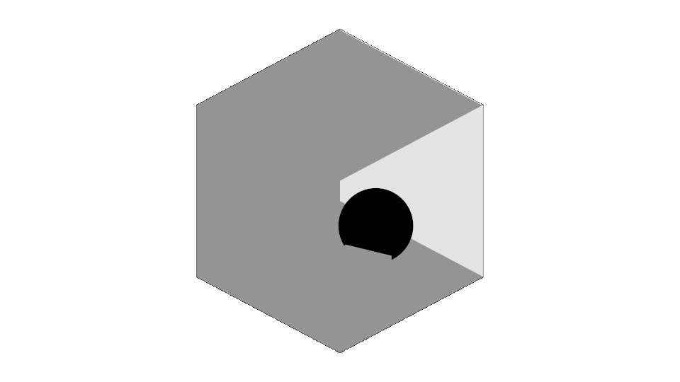
All of these classes of algorithms rely on reusing data, thus when that isn't possible, such as in the case of fast moving objects, highly complex geometry, or areas with little history information, the quality of each method decreases. There are ways to make use of some cached data to help avoid this, such as using irradiance caching to have a better default color as in the case of Minecraft RTX.

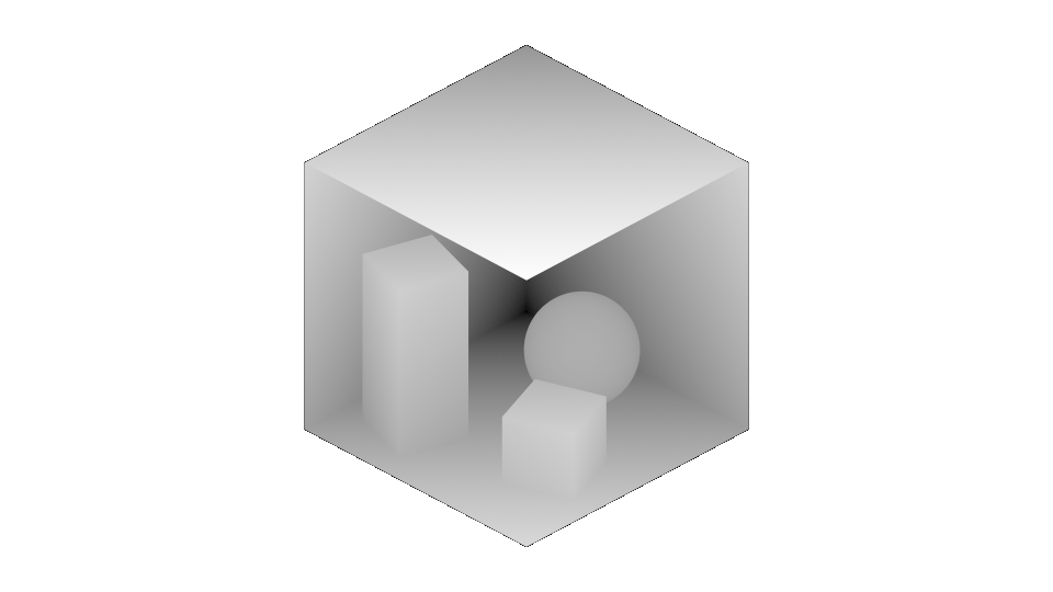
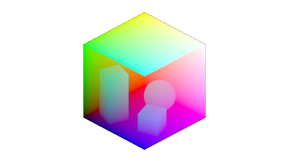
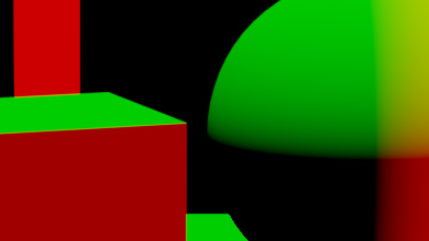
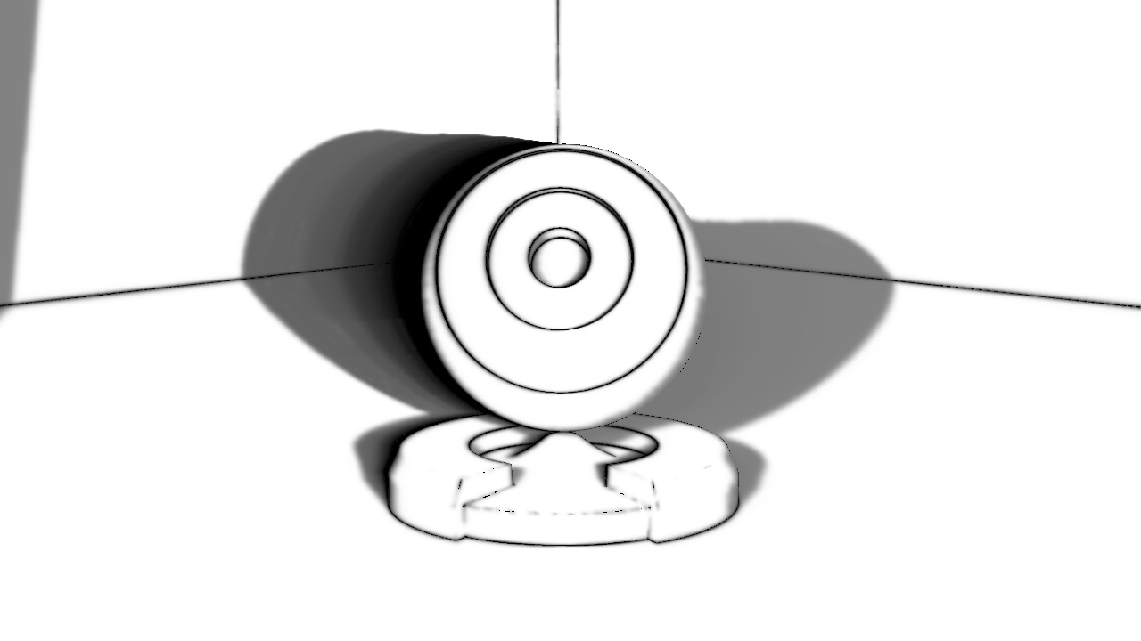
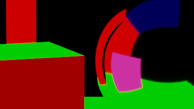
Direct Normals	First Bounce Normals

Spatio-temporal reprojection is also significantly more difficult with reflections, so often times denoisers will rely on first-bounce data, where the normals of a reflective surface, positional data, etc. are based on the first reflection rather than the original surface.

Conclusion

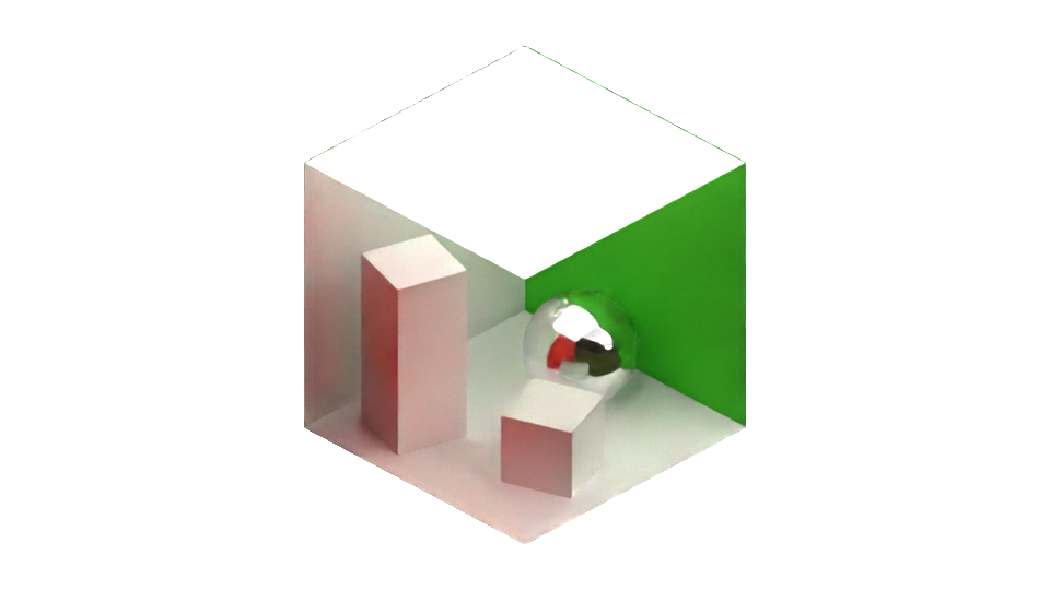
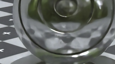
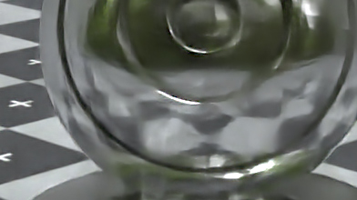
Denoising can help bridge the gap between a low sample per pixel image and ground truth by reusing previous samples through spatio-temporal reprojection - adaptively resampling radiance or statistical information for importance sampling, and using filters such as fast gaussian/bilateral filters or AI techniques like denoising autoencoders and upscaling though super sampling.

While denoising isn't perfect as temporal techniques can introduce a lag in radiance and any filter will introduce some loss of sharpness due to it attempting to blur the original image, guided filters can help maintain sharpness, and adaptively sampling or increasing samples per pixels for each frame can make the difference between denoised and ground truth images negligable. Still, there's no substitute for higher samples per pixel, so experiment with these techniques with different sample per pixel (spp) counts.

Samples

• Dihara Wijetunga (@diharaw94) released a blog post that discusses denoising different aspects of a hybrid renderer.

• NVIDIA released their Real-Time Denoiser for limited review. You can sign up to view it here.

• Interactive Path Tracing and Reconstruction of Sparse Volumes uses a machine learning denoiser to denoise volumes with adaptive sampling.

• Peter Kristof of Microsoft made a really robust DirectX Ray Tracing Ambient Occlusion example with SVGF here.

• The Apple Metal Team released an example of using Metal Performance Shaders, Temporal Anti-Aliasing (MPSTAA), and SVGF (MPSSVGF) to denoise a ray traced scene.

• AMD's FidelityFX SSSR features spatio-temporal reprojection to denoise screen space reflections. Here's their Github. AMD also released several denoisers for reflections and shadows on thisGithub Repo.

• NVIDIA has released an SDK to itegrate Deep Learning Super Sampling here. AMD's Fidelity FX Super resolution is also available for developers to integrate into their applications.

• Ingo Wald (@IngoWald)) released a Optix course which showcases how to use the Optix denoiser here.

• Christof Shied (@c_schied) and Alexey Panteleev (@more_fps) of NVIDIA wrote the denoiser for Quake 2 RTX which is on Github here.

• Microsoft's DirectML Super Resolution Example, while not NVIDIA Deep Learning Super Sampling 2.0 (DLSS 2.0), is similar in that both perform upscaling.

• Xiaoxu Meng released the source of their Neural Bilateral Grid paper here.

• In the University of Pennsylvania's CIS565 course, a number of students, teaching assistants, and former students made awesome projects that implement the latest in denoising research:

  • CUDA SVGF by Zheyuan Xie, Yan Dong, and Weiqi Chen

  • Blockwise Multi-Order Feature Regression for Real-Time Path Tracing Reconstruction (BMFR) by Jiangping Xu, Gangzheng Tong, and Tianming Xu

  • Interactive Reconstruction of Monte Carlo Image Sequences using a Recurrent Denoising Autoencoder by Dewang Sultania & Vaibhav Arcot implemented with Pytorch.

  • ReSTIR in DirectX 12 by Sydney Miller, Sireesha Putcha, Thy Tran.

  • ReSTIR in DirectX 12 by Jilin Liu (@Jilin18043110), Keyi Yu, and Li Zheng.

  • ReSTIR in Vulkan by Xuanyi Zhou, Xuecheng Sun, Jiarui Yan.

Talks

• Chris Wyman's High Performance Graphics 2020 talk on ReSTIR is available here.

• Eric Haines (@pointinpolygon) released Ray Tracing Essentials Part 7: Denoising for Ray Tracing, a great introduction to denoising.

• Tomasz Stachowiak (@h3r2tic) et al. designed the Pica Pica renderer, an amazing reference hybrid renderer featured in Ray Tracing gems. Their talk is available here.

Articles

• Kostas Anagnostou (@KostasAAA) wrote an article describing a method of handling global illumination denoising inspired in part by Metro Exodus.

• Chris Wyman and a number of co-authors for denoising papers at NVIDIA released A Gentle Introduction to ReSTIR: Path Reuse in Real-time.

I've also written blog posts on image based denoising with adaptive spatiotemporal filtering, bilateral filtering, and using machine learning autoencoders, and denoisers of commercial games like Minecraft RTX:

[Dammertz et al. 2010] Edge-Avoiding À-Trous Wavelet Transform for fast Global Illumination Filtering Holger Dammertz (@NeoSpark314), Daniel Sewtz, Johannes Hanika and Hendrik P.A. Lensch High Performance Graphics 2010 jo.dreggn.org

[He et al. 2012] Guided Image Filtering Kaiming He, Jian Sun and Xiaoou Tang 2012 kaiminghe.com

[Mara et al. 2017] An Efficient Denoising Algorithm for Global Illumination Michael Mara, Morgan McGuire (@CasualEffects), Benedikt Bitterli (@tunabrain) and Wojciech Jarosz (@wkjarosz) ACM, High Performance Graphics 2017 cs.dartmouth.edu

[Khademi Kalantari et al. 2013] Removing the Noise in Monte Carlo Rendering with General Image Denoising Algorithms Nima Khademi Kalantari and Pradeep Sen Eurographics 2013 research.nvidia.com

[Khademi Kalantari et al. 2015] A Machine Learning Approach for Filtering Monte Carlo Noise Nima Khademi Kalantari, Pradeep Sen and Steve Bako ACM Transactions on Graphics (TOG) 2015 cvc.ucsb.edu

[R. Alla Chaitanya et al. 2017] Interactive Reconstruction of Monte Carlo Image Sequences using a Recurrent Denoising Autoencoder Chakravarty R. Alla Chaitanya, Anton S. Kaplanyan, Christoph Schied (@c_schied), Marco Salvi (@marcosalvi), Aaron Lefohn, Derek Nowrouzezahrai and Timo Aila ACM 2017 research.nvidia.com

[Vogels et al. 2018] Denoising with Kernel Prediction and Asymmetric Loss Functions Thijs Vogels, Fabrice Rousselle, Brian Mcwilliams, Gerhard Rothlin, Alex Harvill, David Adler, Mark Meyer and Jan Novak ACM, ACM Transactions on Graphics 2018 doi.acm.org

[Wang et al. 2018] A Fully Progressive Approach to Single-Image Super-Resolution Yifan Wang, Federico Perazzi, Brian McWilliams, Alexander Sorkine-Hornung, Olga Sorkine-Hornung and Christopher Schroers CoRR 2018 arxiv.org

[Xu et al. 2019] Adversarial Monte Carlo Denoising with Conditioned Auxiliary Feature Modulation Bing Xu, Junfei Zhang, Rui Wang, Kun Xu, Yong-Liang Yang, Chuan Li and Rui Tang ACM, ACM Transactions on Graphics 2019 adversarial.mcdenoising.org

[Meng et al. 2020] Real-time Monte Carlo Denoising with the Neural Bilateral Grid Xiaoxu Meng, Quan Zheng, Amitabh Varshney, Gurprit Singh and Matthias Zwicker Eurographics 2020 diglib.eg.org

[Işık et al. 2021] Interactive Monte Carlo Denoising using Affinity of Neural Features Mustafa Işık, Krishna Mullia, ‪Matthew Fisher, ‪Jonathan Eisenmann and Michaël Gharbi Siggraph 2021 mustafaisik.net

[Jiang et al. 2022] Fast and High-Quality Image Denoising via Malleable Convolutions Yifan Jiang, Bartlomiej Wronski, Ben Mildenhall (@BenMildenhall), Jonathan T. Barron (@jon_barron), Zhangyang Wang and Tianfan Xue arXiv 2022 yifanjiang.net

[Hasselgren et al. 2020] Neural Temporal Adaptive Sampling and Denoising Jon Hasselgren, Jacob Munkberg, Marco Salvi (@marcosalvi), Anjul Patney and Aaron Lefohn Eurographics 2020 research.nvidia.com

[Verbin et al. 2021] Ref-NeRF: Structured View-Dependent Appearance for Neural Radiance Fields Dor Verbin, Peter Hedman (@peterhedman3), Ben Mildenhall (@BenMildenhall), Todd Zickler, Jonathan T. Barron (@jon_barron) and Pratul Srinivasan (@_pratul_) CVPR 2021 dorverbin.github.io

[Mildenhall et al. 2022] NeRF in the Dark: High Dynamic Range View Synthesis from Noisy Raw Images Ben Mildenhall (@BenMildenhall), Peter Hedman (@peterhedman3), Ricardo Martin-Brualla (@rmbrualla), Pratul Srinivasan (@_pratul_) and Jonathan T. Barron (@jon_barron) CVPR 2022 github.com

[Dong et al. 2015] Image Super-Resolution Using Deep Convolutional Networks Chao Dong, Chen Change Loy, Kaiming He and Xiaoou Tang CoRR 2015 arxiv.org

[Ledig et al. 2016] Photo-Realistic Single Image Super-Resolution Using a Generative Adversarial Network Christian Ledig, Lucas Theis, Ferenc Huszar, Jose Caballero, Andrew P. Aitken, Alykhan Tejani, Johannes Totz, Zehan Wang and Wenzhe Shi CoRR 2016 arxiv.org

[Xiao et al. 2020] Neural Supersampling for Real-time Rendering Lei Xiao, Salah Nouri, Matt Chapman, Alexander Fix, Douglas Lanman and Anton Kaplanyan Facebook Research 2020 research.fb.com

[Mathew Thomas et al. 2022] Temporally Stable Real-Time Joint Neural Denoising and Supersampling Manu Mathew Thomas, Gabor Liktor, Christoph Peters (@MomentsInCG), Sungye Kim, Karthik Vaidyanathan and Angus G. Forbes High Performance Graphics 2022 momentsingraphics.de

[Korein et al. 1983] Temporal Anti-Aliasing in Computer Generated Animation Jonathan Korein and Norman Badler ACM 1983 dl.acm.org

[Yang et al. 2020] A Survey of Temporal Antialiasing Techniques Lei Yang, Shiqiu Liu and Marco Salvi (@marcosalvi) Computer Graphics Forum 2020 onlinelibrary.wiley.com

[Schied 2017] Spatiotemporal Variance-Guided Filtering Christoph Schied (@c_schied) ACM 2017 research.nvidia.com

[Abdollah-shamshir-saz 2018] Voxel Based Hybrid Path Tracing with Spatial Denoising Baktash Abdollah-shamshir-saz (@TooMuchVoltage) i3D 2018 toomuchvoltage.com

[Schied et al. 2018] Gradient Estimation for Real-Time Adaptive Temporal Filtering Christoph Schied (@c_schied), Peters, Christoph and Carsten Dachsbacher ACM 2018 cg.ivd.kit.edu

[Koskela et al. 2019] Blockwise Multi-Order Feature Regression for Real-Time Path Tracing Reconstruction Matias Koskela and Kalle Immonen ACM Transactions on Graphics (TOG) 2019 tut.fi

[Benyoub 2019] Leveraging Ray Tracing Hardware Acceleration In Unity Anis Benyoub (@Auzaiffe) Digital Dragons 2019 auzaiffe.files.wordpress.com

[Liu et al. 2019] Cinematic Rendering in UE4 with Real-Time Ray Tracing and Denoising Edward Liu, Ignacio Llamas, Juan Cañada and Patrick Kelly Ray Tracing Gems 2019 realtimerendering.com

[Veach 1998] Robust Monte Carlo Methods for Light Transport Simulation Eric Veach Stanford University 1998 graphics.stanford.edu

[Pantaleoni 2020] Online Path Sampling Control with Progressive Spatio-Temporal Filtering Jacopo Pantaleoni NVIDIA 2020 arxiv.org

[Bitterli et al. 2020] Spatiotemporal Reservoir Resampling for Real-Time Ray Tracing With Dynamic Direct Lighting Benedikt Bitterli (@tunabrain), Chris Wyman (@_cwyman_), Matt Pharr, Peter Shirley (@Peter_shirley), Aaron Lefohn and Wojciech Jarosz (@wkjarosz) ACM Transaction on Graphics 2020 research.nvidia.com

[Boisse 2021] World-Space Spatiotemporal Reservoir Reuse for Ray-Traced Global Illumination Guillaume Boisse (@guitio2002) Siggraph Asia 2021 gpuopen.com

[Oberberger et al. 2022] Spatiotemporal Variance-Guided Filtering for Motion Blur Max Oberberger, Matthäus G. Chajdas (@NIV_Anteru), Rüdiger Westermann (@MomentsInCG), Sungye Kim, Karthik Vaidyanathan and Angus G. Forbes High Performance Graphics 2022 gpuopen.com

[Tokuyoshi 2022] Tiled Reservoir Sampling for Many-Light Rendering Yusuke Tokuyoshi (@yusuketokuyoshi) 2022 gpuopen.com

[Majercik et al. 2020] Scaling Probe-Based Real-Time Dynamic Global Illumination for Production Zander Majercik, Adam Marrs, Josef Spjut and Morgan McGuire (@CasualEffects) arXiv 2020 arxiv.org

[Talbot et al. 2005] Importance Resampling for Global Illumination Justin Talbot, David Cline and Parris Egbert Eurographics 2005

[Kuznetsov et al. 2018] Deep Adaptive Sampling for Low Sample Count Rendering Alexandr Kuznetsov (@straintensor), Nima Khademi Kalantari and Ravi Ramamoorthi Eurographics 2018 cseweb.ucsd.edu

[Wyman et al. 2021] Rearchitecting Spatiotemporal Resampling for Production Chris Wyman and Alexey Panteleev Eurographics 2021 research.nvidia.com

[Zeng et al. 2021] Temporally Reliable Motion Vectors for Real-time Ray Tracing Zheng Zeng, Edward Liu (@edliu1105), Jinglei Yang, Lu Wang and Ling-Qi Yan Eurographics 2021 sites.cs.ucsb.edu

[Olejnik et al. 2020] Raytraced Shadows in Call of Duty: Modern Warfare Michal Olejnik (@olej3d) and Pawel Koztowski (@PawPawDH) Digital Dragons 2020

[Tokuyoshi 2015] Specular Lobe-Aware Filtering and Upsampling for Interactive Indirect Illumination Yusuke Tokuyoshi (@yusuketokuyoshi) Eurographics 2015 jp.square-enix.com